7.3 Dealing with Cycles
We consider first the problem of finding paths in a graph.
The problem of finding traversals will then be seen as a
straightforward extension of our solution to the problem of finding
paths in a cyclic graph.
Furthermore, we begin by representing graphs directly as Prolog
programs, using an explicit arcs/2 relation to implement a
collection of adjacency lists. This simplifies our path-finding
predicate slightly. Then we move on to consider the case where the
graph is represented as a list of adjacency lists, and so must be
passed around as an argument to the relevant predicates and accessed
with general-purpose list processing predicates like member/2.
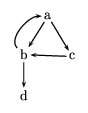
Suppose we have the graph illustrated in figure 7.3.
The set of nodes is just the four element set {a,b,c,d }, and
the arc relation is as given below.
  arcs( a, [b,c] ).
  arcs( b, [a,d] ).
  arcs( c, [b] ).
  arcs( d, [] ).
Figure 7.3: A sample graph.
Naively, we might define a path/3 predicate for this graph in
essentially the same way that we implemented it for trees, that is, by
simply taking the reflexive transitive closure of the arc
relation, compactly encoded by the arcs/2 predicate.
path( X, Y, [] ) :- X = Y.
path( X, Y, P ) :-
    arcs( X, ArcList ),
    member( Z, ArcList ),
    P = [Z|PTail],
    path( Z, Y, PTail ).
However, because there is a loop in the graph, taking us from node
b back to node a, there is an infinite branch in the search
tree for path/3. It gets worse! Because the upward pointing
arc---from b back to a---will be found first by
member/2,
before the downward pointing arc to d, Prolog will find this
infinite branch before it finds any other. And because the clause for
b is earlier than the clause for c in the definition of
arcs/2, note that Prolog will even fail to find a path from
a to c! Clearly, if we want to be able to find paths in an
arbitrary graph, something extra has to be done.
Recalling the example of finite state automata, where we looked at an
automaton that gave us essentially the same problem, we already know
one solution we can apply. We observe that the data structure
definition predicate list/1 will enumerate the lists in order
of increasing length. Given that paths are encoded as lists of
node names, we can redefine the problem
as follows.
list([]).
list([_|L]):- list(L).

?- list(P), path(a,Y,P ).
This technique, where we simulate breadth-first search using
repeated bounded depth-first searches actually has a name: it is
called iterative deepening. Here each successive call to
path/3, in effect,
deepens the search by one level of the search tree.
This solution, by the simulation of iterative deepening,
still finds an infinite number
of (ever longer) paths from a to d, for example.
Almost all of these paths, however, are arrived at by following a loop
in the graph. There are only two ways of reaching d from a
which are truly unique: [a,b,d] and [a,c,b,d]. All the
others are arrived at by following the loop.
What want to do here is not to find all of the paths but rather
all of the cycle-free paths.
A neat way to do this is to note that, after all, we are computing a
path from one node to another. To find out if we have visited a
particular node yet, we should be able to just search the path we are
constructing to see if that node is on it yet. However, path/3 is
not designed in such a way that we can do this intuitively appealing
thing. The part of the path that we have already seen is not
represented as a variable in the code, so we have no access to it; the
only part of the path which we can actually examine is the tail of the
path, the nodes we are going to visit in the future, and this is no
help at all to us! So we modify the code slightly so as to keep track
of the nodes we have actually visited, giving us path/4, below.
path( X, Y, P ) :- % path/3 redefined
    path( X, Y, [X], P ).

path( X, X, Path, Path ).
path( X, Y, PIn, POut ) :-
    arcs( X, L ),
    member( Z, L ),
    nonmember( Z, PIn ), % Been here before?
    path( Z, Y, [Z|PIn], POut ).
This code uses a technique, called accumulator pairs,
which is used everywhere in logic
programming, and which we will examine in some detail when we study
the control and optimization of logic programs. Here we note only
that, while the logical, ``declarative'' semantics of this program may be at this
moment somewhat obscure, it should be reasonably clear what it
does. If we type in a goal like
?- path( a, d, P ).
then this code will begin by initializing the ``path-so-far''
argument to a list containing only the starting point of the
search. Then we call path/4, which does the real work. When we
finally reach our destination, and the base clause applies, then we
simply pass the contents of the ``path-so-far'' argument PIn over
to the output argument POut. This is then passed up to the
calling goal and from it to the goal that called it, and so on up the
chain of recursive calls to path/4 and thence to
path(a,d,P), our original goal. Note that whereas in path/3
we actually built up the path ``on the way up out'' of the recursion,
here we are building it up ``on the way down in.'' This means that at
every point, we can see where we have been so far, by examining the
PIn variable. In this case we do that with a call to
nonmember/2.
As usual, using nonmember/2 requires defining neq/2, in this
case for node names. We can do that in the usual way, with a
collection of unit clauses like ``neq(a,b).'' and so forth. But
neq/2, like any binary relation, can be seen as defining a
graph. This graph has the same set of nodes as the original graph of
figure 7.3, but different arcs. There is an arc between
two nodes in the ``neq-graph'' whenever they are different
nodes. Note that this relation is symmetric, and so technically the
neq-graph is our first example of an undirected graph, but
we can still use the same adjacency list representation scheme, as
follows.
neq( Node1, Node2 ) :-
    neq_arcs( Node1, L ),
    member( Node2, L ).

neq_arcs( a, [b,c,d] ).
neq_arcs( b, [a,c,d] ).
neq_arcs( c, [a,b,d] ).
neq_arcs( d, [a,b,c] ).
With this code in place, we can now safely search in a graph, even
when it contains cycles.
This approach works well when the graph is represented as a Prolog
program, with an arcs/2 predicate defined by a collection of unit
clauses. There is another even neater approach which we can apply when we
represent our graphs using adjacency lists. This approach uses
select/3 to mark a node as visited by actually
removing that node from the graph. Suppose, then, that our
graph is encoded as an instance of the graph/1 predicate.
graph( 1, [a/[b,c],
           b/[a,d],
           c/[b],
           d/[]
          ] ).
(This technique is very useful in general for encoding a set of test
data, especially when the data involve very complex Prolog terms.)
Now we want to define a path/4 predicate so that we can issue
queries like
?- graph( G ), path( a, d, G, P ).
Accordingly, we reimplement path so that it includes an argument position
for the graph itself.
path( From, To, Graph, [From|Path] ) :-
    p( From, To, Graph, Path ).

p( X, Y, _G, [] ) :- X = Y.
p( X, Y, G, [Z|P] ) :-
    select( X/Arcs, G, SmallerG ),
    member( Z, Arcs ),
    p( Z, Y, SmallerG, P ).
Note that each time through the recursive clause of p/4 we reduce
the size of the graph by removing one adjacency record from
it. The select/3 predicate fails when its list argument is empty,
so we can only call clause 2 a finite number of times before it fails
to apply, and clause 1 is
nonrecursive, so we can only call it once in any case.
So no matter which clause of p/4 Prolog selects, the recursion
is bound to terminate. From this one sees immediately that we cannot
possibly get caught in a loop: that would contradict the theorem that
this program is bound to terminate.
Now we can use the same logic to reimplement our depth first traversal
predicate so that it handles (rooted) cyclic graphs. The only
essential difference comes from the fact that this is a traversal
predicate rather than a search predicate. With p/4, if the
call to select/3 fails (the node has already been visited),
then the whole call to p/4 fails, we backtrack and try to
find a different path. With dft/4, if the call to
select/3 fails, we must simply ignore that node and
continue. Therefore we need a call to nonmember_/2 so as to
be certain that we only ignore nodes that we really have already
visited. Similarly, where p/4 calls member/2 to
nondeterministically select one way to extend its current path,
dft/4 must execute a recursion on the entire list of
neighbors, so as to check all ways to traverse the graph.
df_traversal(GIn,[Root|Route]):-
    GIn = [Root/Neighbors|GInRest], % get the root's neighbors
    dft(Neighbors,GInRest,_GOut,Route).

dft([],RemainingG,RemainingG,[]).
dft([N|RestNs],GIn,GOut,[N|Route]):-
    select(N/Nbrs,GIn,SmallerG),
    dft(Nbrs,SmallerG,EvenSmallerG,RfromN),
    dft(RestNs,EvenSmallerG,GOut,RfromRest),
    append(RfromN,RfromRest,Route).
dft([N|RestNs],GIn,GOut,Route):-
    nonmember_(N,GIn), % already visited
    dft(RestNs,GIn,GOut,Route).
The predicate nonmember_/2 which is called in clause 3 of
df_search_2/3 is not quite the same as the predicate
nonmember/2 we have seen before, although it is about as much different
from that predicate as its name implies. The trick is that we are
asking whether or not a node is still present in a graph
and a graph is not a list of nodes, but a list of node/adjacency-list
pairs. The code for nonmember_/2 looks like the following and
assumes that neq/2 has been implemented.
nonmember_( _, [] ).
nonmember_( X, [Y/_|L] ) :-
    neq( X, Y ),
    nonmember_( X, L ).
So we just pull out the node-part of each node/list pair and check
that for inequality with X.