Chapter 5 Lists

Over and over again we will find it useful to arrange our symbolic expressions in sequences. For this purpose we will use the data type list. It is important to recognize, however, that the concept of a sequence is far more general than the concept of a list (by which we mean a particular data structure for representing sequences). So before plunging into the syntax of lists and the construction of list-processing predicates let us first be clear on the intended semantics of this structure. A sequence is a lot like a set, except that its elements appear in a fixed order, and the same symbol can appear any number of times. In order to define what a sequence is, we first have to have available to us an alphabet or lexicon of symbols, which will become the members of our sequences. A sequence of length n over an alphabet S can then be thought of as a function from the first n natural numbers to S . That is, we think of the sequence a₁ a₂ ... a_n as being a way of writing a function A which is such that A(1) = a₁, A(2) = a₂, ..., A(n) = a_n . If n=0 then the sequence is empty. Given any two sequences a₁ ... a_m and b₁ ... b_n we can concatenate them to yield a new sequence a₁ ... a_m b₁ ... b_n .

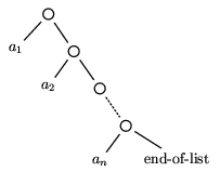
A list, on the other hand, is essentially a uniformly right-branching expression tree such that every node has exactly two daughters, and the last terminal node (i.e., the rightmost terminal node) is labeled by a special official end-of-list symbol. The other nodes can be labeled with anything we please (even other lists). Figure 5.1 illustrates informally the kind of structure we have in mind. Note that the place of an element in a sequence is a function of its depth in the corresponding tree; only two elements have the same depth---a_n and the end-of-list marker---and the end-of-list marker is not an official part of the corresponding sequence, so the mapping from depths to sequence position is indeed a function. Or rather, there is a unique correspondence between ``official'' leaves on the tree and the natural numbers (namely depth) and a unique correspondence between sequence elements and the natural numbers (sequential position), and they both give the same result. So we know (just in case it wasn't already intuitively obvious!) that we can use this sort of tree to represent a sequence.

Figure 5.1: An expression tree with the structure of a list.

5.1 How to write down lists

Lists are so common in Prolog that the language provides a special syntax for them. The empty list is written []. Keep in mind that this is treated as a single constant symbol, although it does not obey the standard rules for constant-names. A non-empty list can be written in one of two ways. The first way of writing a list is this: the list consisting of the expressions a, b and c can be written as [a,b,c]. This way of writing a list makes it appear, in this case, as if it were a flat structure of some sort, that is, an expression tree with three subexpressions. The list [a,b,c,d] would seem to be an expression tree with four subexpressions, and so on. However, this is not the way Prolog actually looks at lists. To Prolog all lists are expressions trees with just two subexpressions, which we refer to as its head and its tail. Abstractly, we can think of lists as being any data type satisfying the following definition.

  list( L ) :- L = [].
  list( L ) :-
      head( L, _ ), 
      tail( L, Tail ),
      list( Tail ).

The head can be anything we like. The tail must be itself a list. The second way of writing lists makes this clearer. The list with head Head and tail Tail can be written [Head|Tail]. This is the notation we use to actually write the ``official'' definition of this new data type.

  list( L ) :- L = [].
  list( L ) :- 
      L = [Hd|Tl], 
      list( Tl ).

Thus lists are recursive data structures, like the notation we defined for natural numbers in the last chapter. Like the natural numbers, there is no a priori bound on the size of a list. The recursive definition allows us to be vague about the length of a list: if the tail of a list is a variable, for example, then it can later be instantiated to another list of any size, or even to a list whose own tail is itself a variable.

Even the ``bar-notation'' [H|T] is different from the kinds of expression trees we are used to. In fact, although Prolog always prints out lists in this more readable notation, internally it treats lists just as it treats all other expression trees. Essentially, Prolog uses a functor `.'/2 in place of the bar-notation. So we have the following three equivalent ways of describing the same data object.

[a,b,c] [a|[b|[c|[]]]] `.'(a, `.'(b, `.'(c, [])))

Note that the bar-notation and the comma-notation can be mixed in the same term:

[a,b,c] = [a|[b,c]] = [a,b|[c]] = [a,b,c|[]]

As usual, `=' means `unifies'. So apparently we have here the exceptional case where several objects which are syntactically distinct actually unify. In fact this is no exception. The rules for unification are defined on Prolog's internal representations (i.e., the dot-notation). All of these expressions are different ``surface'' ways of writing the same ``underlying'' expression tree. ¹ These expressions are strictly cosmetic; they are for you, not for Prolog.

In general, the bar notation is only used when the tail of a list is a variable. Note also that [a,B] and [a|B] are very different objects. The list [a,B] is a list of length 2 whose second element happens to be a variable. The list [a|B] is a list of indeterminate length. The tail of [a,B] is [B]. The tail of [a|B] is just B. Consider, for example, the following short Prolog session.

  ?- [a,B] = [a|C].
  C = [B]
  
  yes

(Question: why didn't I write ``?- [a,B] = [a|B].''?)

Note further that the bar-notation allows us to write terms which are not lists. The term [a|b] is a way of writing a perfectly well-formed expression tree, which could also be written `.'(a,b). However, this expression is not a list. In particular it is not the list [a,b], which corresponds to the expression `.'(a,`.'(b,[])), alias [a|[b]]. As you can see, the two dot-expressions do not unify.

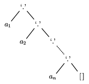
We noted at the beginning of this chapter that the data structure list was a special sort of tree: binary, and uniformly right-branching. So, for example, the list [a1,\ldots,aN] would be represented internally as something like the expression tree in figure 5.2

Figure 5.2: The expression tree representation of the list [a₁,...,a_n] .

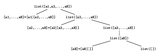
Now consider the proof tree for the goal ?- list([a1,\ldots,aN])., given in figure 5.4, based on the code for list/1 given in figure 5.3. The structure of the proof tree is almost point for point identical to the structure of the expression tree. This should come as no surprise, really. In a sense, the purpose of list/1 is to prove that its input is a list by mapping it piece by piece to a list-structured expression tree. Put another way, the proof of ?- list([a1,\ldots,aN]). represents a search of the input expression tree to verify that every point in that input tree corresponds to a point in a list-shaped expression tree. And, very generally, a search through a particular data element is very likely to reflect the structure of that data element.

        list( [] ).
        list( L ) :- 
            L = [LHead|LTail], 
            list( LTail ).

Figure 5.3: Code for the data type predicate list/1.

Figure 5.4: A proof tree for the goal ?- list([a1,...,aN]).

5.2 Comparing lists and natural numbers

The non-standard aspects of Prolog's list notation may make these structures seem very unfamiliar, but---notation aside---there is a great deal about lists which should seem very familiar from our work with natural numbers. Consider for instance the parallels in the predicates defining the data structures. (See figure 5.5.) Essentially, the empty list corresponds to zero, and the operation of adding a new element on the front of the list corresponds to the operation of applying another instance of the successor function.

        list( L ) :- 
            L = [].
        
        list( L ) :- 
            L = [H|T], 
            list( T ).

        nn( X ) :-
            X = 0.
        
        nn( X ) :- 
            X = s(Y), 
            nn( Y ).

Figure 5.5: Definitions of list/1 and nn/1.

Another example will make the relation even clearer: in figure 5.6 we present the predicate len/2 to compute the length of a list, in successor-notation. Observe that the base clause of len/2 combines the base cases of both nn/1 and list/1. Similarly, the recursive clause of len/2 combines the recursive clauses of nn/1 and list/1. In effect we have taken the two very simple data-type definitions and combined them into a quite useful little predicate. (The predicate length/2 is in fact a built-in predicate in Prolog; it returns the length of a list in standard arabic numerals.)

      len(L,N):-
          L = [],
          N = 0.
      len(L,N):-
          L = [H|T],
          N = s(M),
          len(T,M).

Figure 5.6: Definition of len/2.

If these two data structures are really so similar, then we would expect similar operations to be defined similarly. Take for example addition. The analogous operation on lists is list concatenation, the operation that takes a list [a₁,..., a_m] and a list [b₁,..., b_n] and maps them to a list [a₁,..., a_m, b₁,..., b_n] . (Note that the operation of concatenation yields a list whose length is the sum of the lengths of its operands---this is an essential clue that concatenation really is the generalization of addition to sequences.) The predicate append/3 whose definition is given in figure 5.7 does just this.

          append(L1,L2,L3):-
              L1 = [], 
              L2 = L3.
          append(L1,L2,L3):-
              L1 = [Hd1|Tl1],
              L3 = [Hd3|Tl3],
              Hd1 = Hd3,
              append(Tl1,L2,Tl3).

Figure 5.7: Definition of append/3

As we might expect by now, the base clause of append/3 is essentially the same as that of plus/3, except of course that we have substituted the empty list [] for 0. Furthermore, the recursive clause is largely identical to the recursive clause for plus/3. Borrowing the Å symbol for a moment, we might express the logic of the recursive clause in functional or operational terms as follows.

[X|Y]Å Z = [X|(YÅ Z)]

Though we have invented some notation here without rigorously explaining it, the relation of this fact about concatenation to the corresponding fact about addition:

s(Y) + Z = s(Y + Z)

should be intuitively clear.

Now consider the definition of shorter_than/2, which is true of a pair of lists just in case the first is shorter than the second.

            shorter_than(X,Y):-
                X = [],
                Y = [_|_].
            shorter_than(X,Y):- 
                X = [_|XTail], 
                Y = [_|YTail], 
                shorter_than(XTail,YTail).

Figure 5.8: Definition of shorter_than/2.

The code for shorter_than/2 should be compared to the code for lt/2. In the base clause we use [_|_] in place of s(_); it is a term unifying with all and only the nonempty lists, that is, in a sense, the lists which are strictly greater (``lengthier'') than the empty list. The recursive clauses are also similar. We defined lt/2 based on the fact that if X < Y, then 1+X < 1+Y . Here we define shorter_than/2 based on the fact that if X\prec Y then Z₁. X \prec Z₂. Y (temporarily making use of ``\prec'' to represent the shorter-than relation, and writing the `.'-functor infixed). In words, if X is shorter than Y, then the result of sticking some Z₁ on the front of X is sure to be shorter than the result of sticking a Z₂ on the front of Y. (For example, [a] is clearly shorter than [1,2,3]; so it stands to reason that [X|[a]] should be shorter than [Y|[1,2,3]], and indeed, writing these more normally, it is obvious that [X,a] is shorter than [Y,1,2,3].) Note that we have defined this relation on the number of elements, and not on the number of symbols required to type the list. In the current example, the first list remains shorter than the second even if we instantiate X to [alpha,beta,gamma], and we instantiate Y to alpha.

The moral of this story is that, once we know that two structures are similar in some way, then we immediately inherit many of the procedures we used for the old structure for use with the new structure. Because we are constructing our programs on a firm logical foundation, we do not have to concern ourselves much with the internal workings of append/3, for example. Once we know that concatenation of lists is logically analogous to addition of natural numbers, then we simply make the relevant translations and we are more or less assured that the new predicate will work as we intend it to.

However, there are differences between the list predicates we have defined so far and the natural numbers predicates from the last chapter, and the differences are as instructive as the similarities. Consider now the definition of prefix/2, which we define so that prefix(X,Y) is true of two lists X and Y whenever X is a (proper) prefix of Y, that is, if X is of length n , then the initial n members of Y define a list identical to X. The code is given in figure 5.9. It can readily seen to be a straightforward extension of shorter_than/2. In fact it defines a relation which is a subset of the shorter-than relation. For example, [a,b] is a prefix of [a,b,c,d], and clearly also shorter, but [X,a], though shorter than [X,1,2,3], is not a prefix of the latter.

        prefix(X,Y):-
            X = [],
            Y = [_|_].
        prefix(X,Y):-
            X = [XHead|XTail],
            Y = [YHead|YTail],
            XHead = YHead,
            prefix(XTail,YTail).

Figure 5.9: Definition of prefix/2, for proper prefixes.

Given the parallelism between forming s(X) from a natural number X and forming [H|X] from a list X, we should not be surprised that there is a line-for-line correspondence between shorter_than/2 and lt/2. Note, however, that the definition of prefix/2 requires an extra line, asserting that XHead = YHead. There is more to a list than just the number of members that it has; we care also about the identity of those members. Put another way, there is really only one way to form a larger natural number from a smaller natural number X: add another application of the s-function. But there are as many ways of forming new lists from a list X as there are expression trees---any one of them could serve as the head of the new list [H|X]! Essentially, prefix/2 has more constraints on it than shorter_than/2, which really only cares about the length of a list. Note also that the latter predicate is much less useful in practice than prefix/2.

Another way to look at the same distinction is via several slight modifications of the basic data type definition, given in figure 5.10. The two predicates list_of_nn/1 and list_of_lists/1 are satisfied if their argument is a list all of whose members are of a particular type. Once again, they emphasize the same point we tried to make with prefix/2: unlike natural numbers, lists have members.

        list_of_nn(L):-
            L = [].
        list_of_nn(L):-
            L = [H|T],
            nn(H),
            list_of_nn(T).

        list_of_lists(L) :-
            L = [].
        list_of_lists(L) :-
            L = [H|T],
            list(H),
            list_of_lists(T).

Figure 5.10: Definitions of list_of_Type/1 predicates.

This (rather simple-minded) observation leads us to our next list-processing predicate, presented in figure 5.11. We intend that member(E,L) be true of an expression E and list L whenever E occurs in L.

        member(E,L):- 
            L = [E|_].
        member(E,L):- 
            L = [_|LTail], 
            member(E,LTail).

Figure 5.11: Definition of member/2.

The following innovation appears in the definition of member/2. The base clause is no longer the case where a particular argument unifies with the empty list []. Instead, the recursion ends if the head of the list argument (the second argument) is unifiable with the first argument. This difference is characteristic of predicates whose primary task is searching: processing ends when (or rather, if) the desired term is found. In more logical terms our two sorts of recursion contrast a certain universal flavor with an essentially existential flavor. For example in our data type definitions like nn/1 or list/1 we must examine every element of the data structure to verify that it is legitimate. But in search procedures like member/2 we are more interested in knowing whether or not there exists a term of a certain sort in a particular collection of data. We do not need to consider the whole collection of data to verify this claim. Also note that just as the negation of an existential sentence has a universal flavor, and vice versa, so too if E does not appear in L, then the entire list will be searched before Prolog finally fails, and if a certain term is not a list (e.g., [a|b]), then there is no need to examine the entire term before failing.

5.2.1 Recursion and induction

We can actually formalize this concept of membership in a way that will be useful later on. So far we have looked at recursive definitions in a rather ``top-down'' manner. It is instructive to consider them from a more ``bottom-up'' perspective, as follows. A recursive definition of a set is a way of defining a set by starting with some basic elements, specifying some functions that create new elements out of old ones (the generating functions), and taking our recursively defined set to be the closure of the basic elements under the generating functions. Suppose, then, that we wish to define the two sets NN and Lists. We give the elements of their recursive definitions below.

Definition of NN.
1. Basic(NN) = {0}
2. Gen(NN) = {F _s}, where F _s (t) = s(t) for t Î NN .
Definition of Lists.
1. Basic(Lists) = {[]}
2. Gen(Lists) = {F _exp }, where F _t
  ₁ (t₂) = [t₁| t₂] , for t₁ an expression, t₂ ÎLists .

Observe that the set of generating functions contains only a single element in the definition of NN, but contains an infinite number of elements in the definition of Lists. On the other hand, the generating functions in both definitions are monadic, that is, they take only a single argument. The recursive structure of these elements is in both cases linear. We will see when we cover trees in the next section how we can generalize both natural numbers and (hence) lists so that they are multiply recursive, simply by defining generating functions which are polyadic, i.e., which take more than one argument. In any case, we have here a very compact account of both the similarities and differences between natural numbers and lists: both are based on monadic functions, but one is based on a single monadic function while the other is based on multiple monadic functions. The notion that lists ``have members'' corresponds to the fact that it makes sense to ask, for lists, which generating functions were used to construct them. For natural numbers such a question makes no sense: it is a question with only one possible answer.

There is a form of inductive proof which generalizes mathematical induction to this setting, called structural induction. We will not be so interested in inductive proofs in this course (but they are important for proving the correctness of an implementation!); we examine them here (briefly!) chiefly for the light they shed on constructing recursive predicates, which is our main topic. The principle of structural induction says essentially this: we can prove that a property P holds of all the members of an inductively defined set S by doing the following.

Take all the elements of Basic(S) , and prove that P holds of each of them.
Take all of the generating functions F _{f
_i}/ n (where n as usual gives us the arity of the function) and prove that, whenever t₁,..., t_n have property P , then F _{f
_i} (t₁,..., t_n) has property P .

This approach generalizes to the case where Basic(S) or Gen(S) have more than one member. The idea is to show that the basic elements have a property P and that P is preserved under all the ways of building larger elements.

We have actually already used the principle of structural induction covertly. In Chapter 4 we claimed to be using the principle of mathematical induction (prove P(0) and then prove P(n) Þ P(n+1) ); in fact, strictly speaking, we were using the principle of structural induction (prove P(0) and then prove P(n) Þ P(s(n)), i.e., P( F_s(n)) ). Since s(n) was intended to mean exactly the same thing as n+1 the deceit was harmless, but now that we know the principle of structural induction, we can be more precise about the techniques we have employed.

The relation between recursive definitions of sets and recursively-defined procedures is fairly easy to state at this point. First note that we can associate with any set S a characteristic predicate p_S . We define p_S(x) to be true if and only if (iff) x Î S . Clearly, one way to prove that x Î S is first to identify which generating function F_f/n created x , and which n expressions t₁, ...,t_n F_f/n used to create x. Then we prove that each of the t_i are in S , in the same way. ²

Clearly the definitions of the data-type predicates nn/1, list/1, list_of_nn/1 and list_of_lists/1 are of this sort. The important thing to recognize is that pretty much all procedures manipulating lists or natural numbers in successor notation, for example, follow this pattern. That is, corresponding to the notion of a proof by structural induction we have the important notion of recursion on a structure. For example, we might say that append/3 is implemented using recursion on a list, in particular, recursion on the list that is its first argument. This means that the base case will typically be the base case for the basic data type definition. For example, if a predicate is constructed as a recursion on a list, then its base case will typically be the case where the relevant argument unifies with the empty list. Similarly the recursive step(s) will typically involve some processing of the head element, and recursion on the tail. As noted, this is the case with append/3: the recursion is on the first argument; the base case deals with how to do concatenation when the first argument is []; the recursive step deals with how to do concatenation involving a non-empty first argument in terms of its tail.

We have already noted that the base case for member/2 is not this ``typical'' base case, i.e., though member/2 is implemented as a recursion on a list, its base clause does not represent the case where the list has become empty. So let us examine in some detail how a relation like member/2 fits into this scheme of definition. In the process we may get a better understanding of how this style of definition and proof can apply to cases more complex than just the data type definitions.

For the moment let us think of member/2 as defining a set, namely the set of all lists which have the first argument (call it X) as a member. We can imagine generating such a set in the following way. We do not want to begin the construction with the empty list, because the empty list cannot contain the element we are looking for. We want to choose as our basic elements a set of lists which are in some clear sense the ``smallest'', most elementary possible lists which are guaranteed to possess the property of interest (namely, the property of containing X). We have chosen as our basic elements the set of all lists which have X as their head. This set is infinite, of course, so we might expect that member/2 should have an infinite number of base cases as a result, but in fact this is not true. We appeal here to the magic of Unification, and note that the single term [X|_] represents in a single expression every one of the lists which have X as their head. That is, every list which has X as its head can be represented as [X|_]$\theta$, for some substitution q.

It should be obvious that the generating functions for lists preserve the property of containing X. That is, if t is a list containing X, then F _exp (t) will also be a list containing X, no matter what our choice of exp happens to be. So if we select as the generating functions for the set of ``X-containing lists'' the generating functions for Lists, then we have an almost immediate inductive proof of the correctness of member/2: the set of basic elements has the relevant property, and the property is preserved by the generators. QED.

In fact, this account of member/2 is still insufficient. Technically, member/2 does not define a set of lists, but rather a set of pairs of expressions, the first element of which appears as a member of the second element. Nonetheless our reasoning is essentially sound. We need only make the following modifications. First, our basic elements must be pairs of expressions, and we are interested in just those pairs of expressions which are such that the first element is the head of the second element. Once again, we can appeal to the magic of Unification: in spite of the fact that there are an infinite number of expressions, each of which can be the head of an infinite number of lists, every single one of these pairs unifies with the pair (X,[X|_]), since X is a variable. So indeed our base clause, which we can compactly represent as the unit clause

  member( X, [X|_] ).

does indeed define the set of basic elements that we want.

For the recursive step, we need a set of generating functions which map element-list pairs to element-list pairs, instead of just mapping lists to lists. But this is still simple to do, because we want to map any particular pair (t₁, t₂) to the pair (t₁, F _exp (t₂)), that is, we do not want our generating functions to modify the expression we are looking for in any way. So we can define the generating functions for member-pairs based on the generating functions for lists: for every list generating function F _exp, there is a corresponding member-pair generating function F_exp² which is defined as follows.

exp

: (t₁, t₂) | ® (t₁, F

exp

(t₂))

So, if (X,L) is a member-pair, that is, if member(X,L) is true, then, given an arbitrary exression `_', we can construct a new member-pair (X,[_|L]), that is, member(X,[_|L]) must also be true. And this is exactly how we have implemented the recursive clause of member/2.³

5.3 More members of the `member` family

Another important list-processing predicate, which involves searching, and which is therefore essentially a generalization of member/2, is select/3. The goal select(Item,List,Remainder) succeeds just in case (a) Item is a member of List, and (b) Remainder is a list consisting of all the members of List except for the occurrence of Item that we found.

  select( Item, List, Remainder ) :- 
      List = [Item|Remainder].
  
  select( Item, List, Remainder ) :- 
      List = [ListHead|ListTail],
      Remainder = [ListHead|RemainderTail],
      select( Item, ListTail, RemainderTail ).

Note that the goal ``?- select( X, L, _ ).'' behaves exactly like a call to ``?- member( X, L ).'' The only real difference is that we maintain a record of all the items we found that were not the selected instance of Item. In member/2 we just threw them away.

The next example generalizes member/2 in a different dimension. The predicate which we will name subset/2 assures that every member of one list is also a member of the other.

  subset( L1, L2 ) :- 
      L1 = [],
      list( L2 ).
  subset( L1, L2 ) :- 
      L1 = [L1Hd|L1Tl], 
      member( L1Hd, L2 ), 
      subset( L1Tl, L2 ).

Note that ``subset'' is somewhat of a misnomer here. If L1 and L2 do in fact represent sets, then subset/2 does implement the subset relation. However, it also functions if L1 and/or L2 are not sets, i.e., when some expression occurs more than once in one or both of the lists.

There is another sense in which lists are not sets: they are ordered. Two sets should always be considered equal if they contain the same members, but two lists will only be equal if they contain the same members in the same order. It is sometimes useful to have a predicate which implements a notion of ``sublist'' which preserves order. That is, L1 is a sublist of L2 if all of the elements of L1 occur in L2 in the same order in which they occur in L1. So if L1 were [a,b], then L2 could be [a,37,2,b,4], for example.

  sublist( L1, L2 ) :- 
      L1 = [],
      list( L2 ).
  sublist( L1, L2 ) :- 
      L1 = [L1Hd|L1Tl], 
      L2 = [L2Hd|L2Tl], 
      L1Hd = L2Hd, 
      sublist( L1Tl, L2Tl ).
  sublist( L1, L2 ) :- 
      L2 = [_|L2Tl], 
      sublist( L1, L2Tl ).

This predicate is interesting in that it has two recursive clauses. The first one handles the case where we have found an instance of the head of L1 in L2; the second clause handles the remaining case where we keep looking for an instance of the head of L1 in L2.

Finally, here is another generalization of member/2 which focuses on the orderedness property of lists. The predicate earlier/3 is true of a pair of elements and a list just in case (an instance of) the first member of the pair appears earlier in the list than (an instance of) the second member of the pair.

  earlier( First, Second, List ) :- 
      List = [First|ListTail], 
      member( Second, ListTail ).
  earlier( First, Second, List ) :- 
      List = [_|ListTail], 
      earlier( First, Second, ListTail ).

Observe how this gives us a second notion of ``less than'' related to lists. First we had prefix/2, which was a ``less than'' relation on pairs of lists. Now we have also earlier/2, which is a ``less than'' relation on list elements, relative to a particular list.

5.4 ``Modes'' of Use

In the previous section we defined append/3 as an operation that would concatenate two input lists and output the result. We can think of this usage as the standard mode of operation or just standard mode, for short. However, the advantage of using relations (i.e., predicates) rather than functions is that they are non-directional. Often there are other modes of operation besides the standard one that are useful. Consider for example the following goal.

  ?- append( _Left, [c|_Right], List ).

A little thought should convince you that this goal will succeed in exactly the same cases where

  ?- member( c, List ).

would succeed. That is, they are logically equivalent. In fact, we could have defined member/2 as follows.

  member( X, L ) :- append( _, [X|_], L ).

In this example, we are assuming that append/3 is provided with its third argument as input, rather than its first (and for that matter most of its second) argument. In fact, we can use append/3in this way to match any pattern that we can express as a prefix of a list.

  ?- append( _Left, [c,_,e|_Right], [a,b,c,d,e] ).

So this multi-modal quality of predicates can lead to extremely economical use of code!

Consider another predicate which is in a sense built on this pattern-matching capability of append/3.

  last( Element, List ) :-
      append( _, [Element], List ).

It should be clear on inspection that this predicate is true only when Element is the last element of List. Here the ``pattern'' we are matching is essentially structural, rather than depending on the content of the input list, but the principle of using append/3 in this nonstandard mode as an engine for searching and decomposing lists remains the same.

As a further example, consider how we might redefine earlier/3 in terms of append/3.

  earlier( A, B, List ) :- 
      append( _, [A|AfterA], List ), 
      append( _, [B|_], AfterA ).

Note that the second call to append/3 is exactly the same goal that would be generated by a call to

  ?- member( B, AfterA ).

The first call to append/3 implements a relation which is sort of halfway between member/2 and select/3: we throw away the elements of List which are to the left of A---just like in member/2---but we keep the elements to the right of A---just like in select/3.

Note that the inverse of a function is not guaranteed to be a function. In our terms, if the standard mode of operation of a given predicate is intended to implement a function---with only one solution---there is no guarantee that another mode will still have only one solution. For example there is only one way to concatenate the lists [a,b]and [c,d], but the following goal has a number of solutions.

  ?- append( L1, L2, [a,b,c,d] ).

Sometimes this nondeterminacy can be put to good use. We have seen how to generate the members of a recursively defined set: simply call ``?- nn(X).'' or ``?- list(L).'' for example. We can also very easily construct predicates to generate the elements of arbitrary finite (and not too big!) sets, that is, sets for which generating functions may not exist.

  fruit( X ) :- 
      member( X, [apples, oranges, cherries, bananas] ).

A call to ``?- fruit(F).'' will then generate one after another all the fruits that the computer knows about.⁴ We can use other members of the member/2-family in the same way: select/3 is especially useful in this regard, but subset/2 can also be used to generate the subsets of a given set, which is sometimes necessary.

5.5 Finite State Automata

Now that we have lists, we can represent strings of symbols, e.g., words and sentences. We can define a formal language extensionally as a set of strings. Quite possibly the set will be infinite, but we require that all the strings that make it up be of finite length. And of course we require that our description of this infinite set be merely finite. This requirement, that we be able to describe infinite sets (and infinite objects in general) with finite means is fundamental to both formal linguistics and the theory of computation, and Formal Language Theory has for several decades marked the area where these two sciences meet and interact.

We have seen one way of constructing formal languages, when we first began to construct the language underlying Prolog, and again when we looked at how recursively defined sets could be built up out of basic elements and generating functions. We now look at a slightly different way of building up sets, particularly suited to building up sets of strings.

Informally, a finite state automaton (FSA, for short) is an abstract mathematical description of a machine whose function is to recognize the strings of a particular formal language. A string (sometimes called a ``word'') is considered to be in the language defined by the automaton if and only if it is recognized by the automaton. We assume that the symbols of the input string are written on a tape, which must be finite in length, but can be arbitrarily long. We divide the tape up into cells: each cell contains a single symbol from the input string.

An FSA has a particularly primitive sort of memory. It is built so that at any point in time it is in one of a finite number of states (hence its name). Its ``memory'' is limited to the number of distinct states it can be in. Put another way, an FSA cannot distinguish between all the different ways there might be to get to a particular state. Roughly, all computations that put it in state q₁ are the same as far as the FSA is concerned, but they are all different from all of the computations which would put it in some other state. All it can do is to read the current tape-cell, examine itself to see what state it's in, and then (a) move to the next tape-cell and (b) simultaneously change to a new state. What its new state will be is determined by a transition relation, which is really the heart and soul of the language-definition that the FSA encodes.

An FSA defines a language in the following way. One of its states is distinguished as the start state. Then a subset of states (possibly including the start state) are designated as possible final states. We start the machine in its designated start state, looking at the first cell of the input tape. If there is a sequence of transitions from state to state such that, after scanning the tape, the FSA is in one of its designated final states, then the string written on the tape is in the language recognized by the FSA. Otherwise it is not. (There are actually two ways for a string to be ruled out: the FSA can end up in a non-final state, or it can at some point in the middle of the string find itself in a state from which there is no possible transition, given the current symbol.)

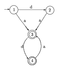
FSAs are usually depicted as in figure 5.12. Circles represent states; they are numbered so that we can refer to particular states easily. Double circles represent final states. Arcs represent possible transitions, and labels on the arcs are taken from the underlying alphabet or lexicon of the language. So, for example, if our machine of figure 5.12 is in state 3 and reads a `d', then it moves to state 4. The arc with no label and no state-of-origin indicates the designated start state (state 1, in this case).

Figure 5.12: A finite state automaton for recognizing a very childish language.

We can see that, given the string `dada', this automaton will start in state 1, scanning a `d'. The only possible transition is then to state 2; now the FSA is in state 2, scanning an `a', so the only possible transition is to state 3, whence reading a `d' takes the FSA to state 4, whence reading another `a' takes it back to state 3. There is no more input, and the machine is in a final state, so `dada' is in the language that it recognizes.

The string `d' would ``strand'' the machine in state 2, a non-final state, and the string `dadd' would strand the machine in state 4 reading a `d', for which no transition is defined. These strings are therefore not in the language.

More formally, a finite state automaton A is defined as below.

A = áS,Q,q₀,F,dñ

S is the underlying alphabet (S = {d,a} in this example), Q={1,2,3,4} is the set of states, q₀=1 is the start state, F={3,4} are the final states and d is the transition relation.

d Í Q× S × Q

We can also think of d as a transition function which maps state-symbol pairs to sets of states.

^d(q,s) = {q' | d(q,s,q') }

Note that if the output of the ^d function is always a singleton set, that is, a set with only one member, then the automaton is deterministic. FSA's do not need to be deterministic: from any given state, reading any given symbol, it is perfectly legal to have several transitions. Note, however, that the automaton of figure 5.12 is deterministic.

It is usual to define an extended transition relation which takes strings of symbols instead of individual symbols as its second argument. For a Î S , w Î S^* and e the empty string, we have the following definition of d^* .

d^*(q_i,e,q_j)	Û	q_j = q_i
d^*(q_i,aw,q_j)	Û	($ q_k)[d(q_i,a,q_k) Ù d^*(q_k,w,q_j)]

The relation d^* is thus essentially the reflexive, transitive closure of the relation d. Accordingly, a string w is in the language recognized by A (denoted L(A) ) just in case

d^*(q₀,w,q) Ù q Î F. (5.1)

From this formal definition it is an almost trivial matter to implement a finite state automaton in Prolog. First, we implement the transition relation using the predicate delta/3, essentially by just reading off the arcs in figure 5.12.

  delta( 1, d, 2 ).
  delta( 1, a, 3 ).
  delta( 2, a, 3 ).
  delta( 3, d, 4 ).
  delta( 4, a, 3 ).

Then we define the start and end states appropriately.

  start_state(1).

  final_state(3).
  final_state(4).

We will use lists to encode strings, so the empty string e becomes the empty list [] and the string aw is represented as a list [A|W]. So we can define delta_star/3 accordingly.

  delta_star( Q, [], Q ).
  delta_star( Q0, [A|W], Q ) :-
      delta( Q0, A, Q1 ),
      delta_star( Q1, W, Q ).

Finally, given our compact definition of recognition in (5.1), we can implement recognize/1 as follows.

  recognize( String ) :- 
      start_state( Q0 ), 
      delta_star( Q0, String, Q ), 
      final_state( Q ).

And that is that. Now for example we can type in goals like

  ?- recognize( [a,d,a,d,a] ).

and have Prolog tell us whether or not the given input string is in the language of our automaton or not. For example, the above goal should succeed, but the following goal should fail.

  ?- recognize( [a,d,a,d,d] ).

Note, before we continue, that if we wish to change the language defined by the automaton, we need only change the clauses defining delta/3, start_state/1 and final_state/1. The clauses defining delta_star/3 and recognize/1 come from the general definition of what it means to be a Finite State Automaton, and remain the same for all FSA's that we might want to implement.

5.5.1 On Enumerating Infinite Sets

As you might expect by now, we can use recognize/3 not only to recognize strings input by the user, but also to generate all the strings of the language.

  ?- recognize( X ).
  
  X = [d,a] ; 
  X = [d,a,d] ; 
  X = [d,a,d,a] ;

and so on until you lose patience.

Well, this is almost true. In fact there is a technical sense in which Prolog will not enumerate all the strings of the language, and it has nothing to do with the infiniteness of the set involved. ``Enumerate'' means something special in mathematics. In particular it means that if we generate a sequence, even though the sequence may be infinite, any particular member of that sequence will be listed after a finite amount of time. This is clearly true of our definition of nn/1, for example. For any arbitrary natural number n its successor-notation-name will be generated in approximately n steps. Here however we are in a different situation. The ``enumeration'' order for strings in this automaton is

da, dad, dada, ..., a, ad, ada, ...

where each occurrence of ``...'' stands for an infinitely long sequence. Clearly, then, the string a will not in fact be listed after any finite amount of time.

Of course this language has only countably many members. That is, there is no sense in which this language is somehow twice as big as the set of natural numbers, for example, just because the given automaton, left to its own devices, will generate the language as two infinite sequences instead of one. The problem is not with the language but with the order in which we list its members. If we listed them as

a, da, ad, dad, ada, dada, adad, ... (5.2)

for example then there would be no problem. That is, we list all of the strings of length 1, then all the strings of length 2, and so on. In this case it should be clear that any string of the language will in fact be listed after some finite number of steps.

In fact we can accomplish this reordering without any deep modifications to Prolog or our program. We simply issue the goal

  ?- len( L, _ ), recognize( L ).

The calls to len/2 will generate list templates (lists filled with anonymous variables) in order of length: first [], then [_], then [_,_], and so forth. Then recognize/1 will see if there are any strings in the language that match these templates. Keep in mind that Prolog, when backtracking to find more solutions, retries the most recent goal first, so only when it has run out of strings of length k to recognize will it backtrack all the way to len/2 and start work on strings of length k+1 . This will in fact give us the enumeration order in (5.2), which is a proper enumeration.

Note that we have actually accomplished something a little deeper than just smoothing out the generating behavior of recognize/1. Recall that normally Prolog performs a depth first search of its search tree, and indeed it is doing so here as well. But the depth first search of the search tree for the goal

  ?- len( L, _ ), recognize( L ).

corresponds exactly to the breadth-first traversal of the search tree for the simpler goal

  ?- recognize( L ).

We have in effect tricked Prolog into running breadth-first instead of depth-first!

5.5.2 A linguistically deeper automaton

Suppose we wish to define a formal language which approximates a natural language with the following phonological property. In this language, coronal stops (t and d) appear to be ``palatalized'' before front vowels (i and e). That is, a t might appear in a word like atogu, but instead of a word like *ategu, we would see only achegu. Assume further that this language has only CV syllables, with the added possibility of words beginning with a vowel and ending in a consonant. Note that it follows from this description that words cannot end in affricates. So chit is a word but *chich is not.

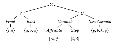
Figure 5.13: The alphabet S.

Let A be a S-automaton, where S is defined as in figure 5.13, defined by the following Prolog clauses.

  %states( [1,2.1,2.2,3,4.1,4.2] ).

  start_state( 1 ).

  final_state( 3 ).
  final_state( 4.2 ).

and the transition relation delta/3 is defined as follows.

  delta(1,X,2.1) :- affricate( X ).
  delta(1,X,2.1) :- non_coronal( X ).
  delta(1,X,2.2) :- stop( X ).
  delta(1,X,2.2) :- non_coronal( X ).
  delta(1,X,3) :- vowel( X ).
  delta(2.1,X,3) :- front( X ).
  delta(2.2,X,3) :- back( X ).
  delta(3,X,4.1) :- affricate( X ).
  delta(3,X,4.1) :- non_coronal( X ).
  delta(3,X,4.2) :- stop( X ).
  delta(3,X,4.2) :- non_coronal( X ).
  delta(4.1,X,3) :- front( X ).
  delta(4.2,X,3) :- back( X ).

The transition relation is based on the automaton for the ``dada-language'' which we examined previously. That automaton gives us our basic CV structure. We need to split states 2 and 4 to handle the different types of vowels and their effects on consonants, so we now have states 2.1, 2.2, 4.1 and 4.2. Note that state 4.2 is a final state, but state 4.1 is not: this prevents us from ending a word in an affricate consonant. Note also that this automaton is nondeterministic: in states 1 and 3, reading a non-coronal consonant, automaton A can move in either of two directions, since a non-coronal consonant is free to occur before either type of vowel.

The auxiliary clauses which we have used to name subcategories of the alphabet S are defined as follows.

  vowel( X ) :- front( X ).
  vowel( X ) :- back( X ).

  front( i ).    front( e ).

  back( a ).    back( o ).     back( u ).

  consonant( X ) :- coronal( X ).
  consonant( X ) :- non_coronal( X ).

  coronal( X ) :- affricate( X ).
  coronal( X ) :- stop( X ).

  affricate( ch )    affricate( j ).
  
  stop( t ).     stop( d ).
  
  non_coronal( p ).    non_coronal( b ).
  non_coronal( k ).    non_coronal( g ).

Exercise: Japanese exhibits a similar, but slightly different and slightly more complex phonological process. There (simplifying tremendously) coronal stops are replaced by these palatal affricates (t ¾® ch, d ¾® j ) before i, and they are replaced by alveolar affricates before u (t¾®ts, d¾®dz, something like that anyway). How would you modify automaton A so that it recognized/generated legal words of `pseudo-Japanese'?

1: In fact it seems wrong to refer to them as ``expressions''. We probably should reserve the name ``expression'' for things which obey the rules we set out earlier. The above objects are then something like different ``ways of writing an expression''.
2: If this reminds you of the relation between a grammar and a recognizer, it should! The rules of a grammar can be seen as a set of generating functions, with the elements of the lexicon as basic elements. Capitalizing on this similarity we can greatly extend the power of our grammatical formalisms, by incorporating a wider array of generating functions, while still being able to use the computational techniques developed for simple context-free grammars.
3: There is one further detail to consider: we have assumed so far that in all of our pairs of expressions, the second one was a list. In fact, our code does nothing to enforce this. For example, the goal ?- member( a, [a|b] ). will succeed (though member(b,[a|b]) will not). Our formal definitions reflect this; in particular, our definition of the basic elements says they just consist of all of the pairs of expressions such that the first element is the head of the second element, that is, such that the second element is the result of `cons'-ing the first element onto some other expression. It is easy to modify the code for member/2 so as to enforce that the second argument is a list, but this is not in general worth the extra computational effort, and we almost always will just use this ``relaxed'' or ``approximate'' definition in practice.
4: For the fun of it, you might try the following goal: ?- fruit(X), write(X), fail.

This document was translated from L^AT_EX by H^EV^EA.